Wednesday, September 7, 2016

Fill data automatically in worksheet cells

Fill data automatically in worksheet cells

Instead of entering data manually on a worksheet, you can use the Auto Fill feature to fill cells with data that follows a pattern or that is based on data in other cells.
This article does not explain how to enter data manually or enter data simultaneously on multiple worksheets. For information about how to manually enter data, see the article Enter data manually in worksheet cells.

What do you want to do?

Automatically repeat values that already exist in the column
Turn automatic completion of cell values on or off
Fill data into adjacent cells by using the fill handle
Show or hide the fill handle
Drag the fill handle to fill data into adjacent cells
Turn Auto Fill Options on or off
Fill data into adjacent cells by using the Fill command
Fill formulas into adjacent cells
Fill in a series of numbers, dates, or other built-in series items
Fill cells with a series by using the fill handle
Fill cells with a series by using the Fill command
Examples of series that you can fill
Fill data by using a custom fill series
Use a custom fill series based on an existing list of items
Use a custom fill series based on a new list of items
Edit or delete a custom fill series

Automatically repeat values that already exist in the column

If the first few characters that you type in a cell match an existing entry in that column, Excel automatically enters the remaining characters for you. Excel automatically completes only those entries that contain text or a combination of text and numbers. Entries that contain only numbers, dates, or times are not automatically completed.
After Excel completes what you started typing, do one of the following:
  • To accept a proposed entry, press Enter.
    The completed entry exactly matches the pattern of uppercase and lowercase letters of the existing entry.
  • To replace the automatically entered characters, continue typing.
  • To delete the automatically entered characters, press Backspace.
Note: 
  • Excel completes an entry only when the cursor is at the end of the current cell contents.
  • Excel bases the list of potential AutoComplete entries on the column that contains the active cell. Entries that are repeated within a row are not automatically completed.
Top of Page

Turn automatic completion of cell values on or off

If you don't want Excel to automatically complete cell values, you can turn off this feature.
  1. Click the File tab, and then click Options.
  2. Click Advanced, and then under Editing options, select or clear the Enable AutoComplete for cell values check box to turn automatic completion of cell values on or off.
Top of Page

Fill data into adjacent cells by using the fill handle

To quickly fill in several types of data series, you can select cells and drag the fill handle Fill handle . To use the fill handle, you select the cells that you want to use as a basis for filling additional cells, and then drag the fill handle across or down the cells that you want to fill.
By default, the fill handle is displayed, but you can hide it, or show it if it's hidden.
After you drag the fill handle, the Auto Fill Options button is displayed. If you don't want to display the Auto Fill Options button every time that you drag the fill handle, you can turn it off. Likewise, if the Auto Fill Options button does not appear when you drag the fill handle, you might want to turn it on.

Show or hide the fill handle

  1. Click the File tab, and then click Options.
  2. Click Advanced, and then under Editing options, select or clear the Enable fill handle and cell drag-and-drop check box to show or hide the fill handle.
  3. To avoid replacing existing data when you drag the fill handle, make sure that the Alert before overwriting cells check box is selected. If you don't want to see a message about overwriting nonblank cells, you can clear this check box.
Top of Page

Drag the fill handle to fill data into adjacent cells

  1. Select the cells that contain the data that you want to fill into adjacent cells.
  2. Drag the fill handle across the cells that you want to fill.
  3. To change how you want to fill the selection, click Auto Fill Options Button image , and then click the option that you want.
    For example, you can choose to fill just cell formats by clicking Fill Formatting Only, or you can choose to fill just the contents of a cell by clicking Fill Without Formatting.
Note: If you drag the fill handle up or to the left of a selection and stop in the selected cells without going past the first column or the top row in the selection, Excel deletes the data within the selection. You must drag the fill handle out of the selected area before releasing the mouse button.
Top of Page

Turn Auto Fill Options on or off

  1. Click the File tab, and then click Options.
  2. Click Advanced, and then under Cut, copy, and paste, select or clear the Show Paste Options button when content is pasted check box to turn this option on or off.
Top of Page

Fill data into adjacent cells by using the Fill command

You can use the Fill command to fill the active cell or a selected range with the contents of an adjacent cell or range.
  1. Do one of the following:
    • To fill the active cell with the contents of an adjacent cell, select an empty cell that is below, to the right, above, or to the left of the cell that contains the data that you want to use to fill the empty cell.
    • To fill multiple adjacent cells, select the cell with the contents you want to fill and the adjacent cells into which you want to fill the content.
  2. On the Home tab, in the Editing group, click Fill, and then click Down, Right, Up, or Left.
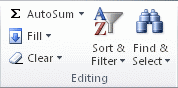
Excel  Ribbon Image
Keyboard shortcut    To quickly fill a cell with the contents of an adjacent cell, you can press Ctrl+D to fill from the cell above or Ctrl+R to fill from the cell to the left.
Top of Page

Fill formulas into adjacent cells

  1. Select the cell that contains the formula that you want to fill into adjacent cells.
  2. Drag the fill handle Fill handle across the cells that you want to fill.
  3. To choose how you want to fill the selection, click Auto Fill Options Button image , and then click the option that you want.
    Note: If automatic workbook calculation is not enabled, formulas will not recalculate when you fill cells. To check your workbook calculation options, do the following:
  4. Click the File tab.
  5. Under Excel, click Options, and then click the Formulas category.
  6. Under Calculation options, look under Workbook Calculation.
    • Automatic    Formulas automatically recalculate.
    • Automatic except for data tables    Formulas recalculate, unless the formula is in a data table.
    • Manual    Formulas never recalculate automatically.
    • Recalculate workbook before saving    This option is available only if Workbook Calculation is set to Manual. If this check box is selected, formulas do not automatically recalculate until you save the workbook. Note that several other actions can cause the workbook to be saved, such as using the Send To command.
      Note: 
  7. You can also fill the active cell with the formula of an adjacent cell by using the Fill command (on the Home tab in the Editing group), or by pressing Ctrl+D to fill a cell below or Ctrl+R to fill a cell to the right of the cell containing the formula.
  8. You can automatically fill a formula downward, for all adjacent cells that it applies to, by double-clicking the fill handle of the first cell that contains the formula. For example, cells A1:A15 and B1:B15 contain numbers, and you type the formula =A1+B1 in cell C1. To copy that formula into cells C2:C15, select cell C1 and double-click the fill handle.
Top of Page

Fill in a series of numbers, dates, or other built-in series items

You can quickly fill cells in a range with a series of numbers or dates, or with a built-in series for days, weekdays, months, or years by using the fill handle or the Fill command.

Fill cells with a series by using the fill handle

  1. Select the first cell in the range that you want to fill.
  2. Type the starting value for the series.
  3. Type a value in the next cell to establish a pattern.
    For example, if you want the series 1, 2, 3, 4, 5..., type 1 and 2 in the first two cells. If you want the series 2, 4, 6, 8..., type 2 and 4. If you want the series 2, 2, 2, 2..., you can leave the second cell blank.
  4. Select the cell or cells that contain the starting values.
  5. Drag the fill handle Fill handle across the range that you want to fill.
    To fill in increasing order, drag down or to the right. To fill in decreasing order, drag up or to the left.
    Note: 
  6. You can also specify the type of series by using the right mouse button to drag the fill handle over the range and then clicking the appropriate command on the shortcut menu. For example, if the starting value is the date JAN-2007, click Fill Months for the series FEB-2007, MAR-2007, and so on; or click Fill Years for the series JAN-2007, JAN-2008, and so on.
  7. If the selection contains numbers, you can control the type of series that you want to create.
  8. You can suppress series AutoFill by holding down Ctrl as you drag the fill handle of a selection of two or more cells. The selected values are then copied to the adjacent cells, and Excel does not extend a series.
Top of Page

Fill cells with a series by using the Fill command

  1. Select the first cell in the range that you want to fill.
  2. Type the starting value for the series.
  3. On the Home tab, in the Editing group, click Fill, and then click Series.
    Excel  Ribbon Image
  4. Under Type, click one of the following options:
    • Linear    Creates a series that is calculated by adding the value in the Step value box to each cell value in turn.
    • Growth    Creates a series that is calculated by multiplying the value in the Step value box by each cell value in turn.
    • Date    Creates a series that fills date values incrementally by the value in the Step value box and is dependent on the unit specified under Date unit.
    • AutoFill    Creates a series that produces the same results as dragging the fill handle.
  5. To establish a pattern for the series, in the Step value and Stop value boxes, type the values you want.
Top of Page

Examples of series that you can fill

When you fill a series, the selections are extended as shown in the following table. In this table, items that are separated by commas are contained in individual adjacent cells on the worksheet.
Initial selection Extended series
1, 2, 34, 5, 6,...
9:0010:00, 11:00, 12:00,...
MonTue, Wed, Thu,...
MondayTuesday, Wednesday, Thursday,...
JanFeb, Mar, Apr,...
Jan, AprJul, Oct, Jan,...
Jan-07, Apr-07Jul-07, Oct-07, Jan-08,...
15-Jan, 15-Apr15-Jul, 15-Oct,...
2007, 20082009, 2010, 2011,...
1-Jan, 1-Mar1-May, 1-Jul, 1-Sep,...
Qtr3 (or Q3 or Quarter3)Qtr4, Qtr1, Qtr2,...
text1, textAtext2, textA, text3, textA,...
1st Period2nd Period, 3rd Period,...
Product 1Product 2, Product 3,...
Top of Page

Fill data by using a custom fill series

To make entering a particular sequence of data (such as a list of names or sales regions) easier, you can create a custom fill series. A custom fill series can be based on a list of existing items on a worksheet, or you can type the list from scratch. You cannot edit or delete a built-in fill series (such as a fill series for months and days), but you can edit or delete a custom fill series.
Note: A custom list can only contain text or text mixed with numbers.

Use a custom fill series based on an existing list of items

  1. On the worksheet, select the list of items that you want to use in the fill series.
  2. Click the File tab, and then click Options.
  3. Click Advanced, and then under General, click the Edit Custom Lists button.
  4. Verify that the cell reference of the list of items that you selected is displayed in the Import list from cells box, and then click Import.
    The items in the list that you selected are added to the Custom lists box.
  5. Click OK twice.
  6. On the worksheet, click a cell, and then type the item in the custom fill series that you want to use to start the list.
  7. Drag the fill handle Fill handle across the cells that you want to fill.
Top of Page

Use a custom fill series based on a new list of items

  1. Click the File tab, and then click Options.
  2. Click Advanced, and then under General, click Edit Custom Lists.
  3. In the Custom lists box, click NEW LIST, and then type the entries in the List entries box, starting with the first entry.
  4. Press Enter after each entry.
  5. When the list is complete, click Add, and then click OK twice.
  6. On the worksheet, click a cell, and then type the item in the custom fill series that you want to use to start the list.
  7. Drag the fill handle Fill handle across the cells that you want to fill.
Top of Page

Edit or delete a custom fill series

  1. Click the File tab, and then click Options.
  2. Click Advanced category, and then under General, click Edit Custom Lists.
  3. In the Custom lists box, select the list that you want to edit or delete, and then do one of the following:
    • To edit the fill series, make the changes that you want in the List entries box, and then click Add.
    • To delete the fill series, click Delete.


Wrap text in a cell

Wrap text in a cell

Microsoft Excel can wrap text so it appears on multiple lines in a cell. You can format the cell so the text wraps automatically, or enter a manual line break.

What do you want to do?

Wrap text automatically
Enter a line break

Wrap text automatically

  1. In a worksheet, select the cells that you want to format.
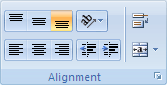
  2. On the Home tab, in the Alignment group, click Wrap Text Button image .
    Excel Ribbon Image
    Notes: 
    • Data in the cell wraps to fit the column width, so if you change the column width, data wrapping adjusts automatically.
    • If all wrapped text is not visible, it may be because the row is set to a specific height or that the text is in a range of cells that has been merged.

Adjust the row height to make all wrapped text visible

  1. Select the cell or range for which you want to adjust the row height.
  2. On the Home tab, in the Cells group, click Format.
    The Cells group on the Home tab
  3. Under Cell Size, do one of the following:
    • To automatically adjust the row height, click AutoFit Row Height.
    • To specify a row height, click Row Height, and then type the row height that you want in the Row height box.
      Tip:  You can also drag the bottom border of the row to the height that shows all wrapped text.
Top of Page

Enter a line break

To start a new line of text at any specific point in a cell:
  1. Double-click the cell in which you want to enter a line break.
    Tip:  You can also select the cell, and then press F2.
  2. In the cell, click the location where you want to break the line, and press Alt+ Enter.


Fix text-formatted numbers by applying a number format

Fix text-formatted numbers by applying a number format

In some cases, numbers in a worksheet are actually formatted and stored in cells as text, which can cause problems with calculations or produce confusing sort orders. This issue sometimes occurs after you import or copy data from a database or other external data source.
Numbers that are formatted as text are left-aligned instead of right-aligned in the cell, and are often marked with an error indicator.

What do you want to do?

Technique 1: Convert text-formatted numbers by using Error Checking
Technique 2: Convert text-formatted numbers by using Paste Special
Technique 3: Apply a number format to text-formatted numbers
Turn off Error Checking

Technique 1: Convert text-formatted numbers by using Error Checking

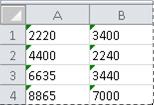
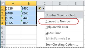
If you import data into Excel from another source, or if you type numbers into cells that were previously formatted as text, you may see a small green triangle in the upper-left corner of the cell. This error indicator tells you that the number is stored as text, as shown in this example.
Cells with green error indicator in upper-left corner
If this isn't what you want, you can follow these steps to convert the number that is stored as text back to a regular number.
  1. On the worksheet, select any single cell or range of cells that has an error indicator in the upper-left corner.
    How to select cells, ranges, rows, or columns
    To select Do this
    A single cellClick the cell, or press the arrow keys to move to the cell.
    A range of cellsClick the first cell in the range, and then drag to the last cell, or hold down Shift while you press the arrow keys to extend the selection.
    You can also select the first cell in the range, and then press F8 to extend the selection by using the arrow keys. To stop extending the selection, press F8 again.
    A large range of cellsClick the first cell in the range, and then hold down Shift while you click the last cell in the range. You can scroll to make the last cell visible.
    All cells on a worksheetClick the Select All button.
    Select All button
    To select the entire worksheet, you can also press Ctrl+A.
    If the worksheet contains data, Ctrl+A selects the current region. Pressing Ctrl+A a second time selects the entire worksheet.
    Nonadjacent cells or cell rangesSelect the first cell or range of cells, and then hold down Ctrl while you select the other cells or ranges.
    You can also select the first cell or range of cells, and then press Shift+F8 to add another nonadjacent cell or range to the selection. To stop adding cells or ranges to the selection, press Shift+F8 again.
    You cannot cancel the selection of a cell or range of cells in a nonadjacent selection without canceling the entire selection.
    An entire row or columnClick the row or column heading.
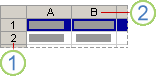
    Worksheet headings
    1. Row heading
    2. Column heading
    You can also select cells in a row or column by selecting the first cell and then pressing Ctrl+Shift+Arrow key (Right Arrow or Left Arrow for rows, Up Arrow or Down Arrow for columns).
    If the row or column contains data, Ctrl+Shift+Arrow key selects the row or column to the last used cell. Pressing Ctrl+Shift+Arrow key a second time selects the entire row or column.
    Adjacent rows or columnsDrag across the row or column headings. Or select the first row or column; then hold down Shift while you select the last row or column.
    Nonadjacent rows or columnsClick the column or row heading of the first row or column in your selection; then hold down Ctrl while you click the column or row headings of other rows or columns that you want to add to the selection.
    The first or last cell in a row or columnSelect a cell in the row or column, and then press Ctrl+Arrow key (Right Arrow or Left Arrow for rows, Up Arrow or Down Arrow for columns).
    The first or last cell on a worksheet or in a Microsoft Office Excel tablePress Ctrl+Home to select the first cell on the worksheet or in an Excel list.
    Press Ctrl+End to select the last cell on the worksheet or in an Excel list that contains data or formatting.
    Cells to the last used cell on the worksheet (lower-right corner)Select the first cell, and then press Ctrl+Shift+End to extend the selection of cells to the last used cell on the worksheet (lower-right corner).
    Cells to the beginning of the worksheetSelect the first cell, and then press Ctrl+Shift+Home to extend the selection of cells to the beginning of the worksheet.
    More or fewer cells than the active selectionHold down Shift while you click the last cell that you want to include in the new selection. The rectangular range between the active cell and the cell that you click becomes the new selection.
    To cancel a selection of cells, click any cell on the worksheet.
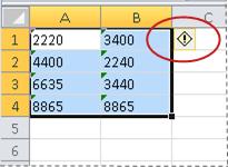
  2. Next to the selected cell or range of cells, click the error button that appears.
    Error button
  3. On the menu, click Convert to Number. (If you want to simply get rid of the error indicator without converting the number, click Ignore Error.)
    Convert to Number command
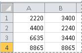
    This action converts the numbers that are stored as text back to numbers.
    Converted numbers
    Once you have converted the numbers formatted as text into regular numbers, you can change the way the numbers appear in the cells by applying or customizing a number format. For more information, see Available number formats.
Top of Page

Technique 2: Convert text-formatted numbers by using Paste Special

In this technique, you multiply each selected cell by 1 in order to force the conversion from a text-formatted number to a regular number. Because you're multiplying the contents of the cell by 1, the result in the cell looks identical. However, Excel actually replaces the text-based contents of the cell with a numerical equivalent.
  1. Select a blank cell and verify that its number format is General.
    How to verify the number format
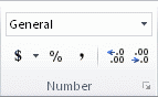
    • On the Home tab, in the Number group, click the arrow next to the Number Format box, and then click General.
      Excel  Ribbon Image
  2. In the cell, type 1, and then press ENTER.
  3. Select the cell, and then press Ctrl+C to copy the value to the Clipboard.
  4. Select the cells or ranges of cells that contain the numbers stored as text that you want to convert.
    How to select cells, ranges, rows, or columns
    To select Do this
    A single cellClick the cell, or press the arrow keys to move to the cell.
    A range of cellsClick the first cell in the range, and then drag to the last cell, or hold down Shift while you press the arrow keys to extend the selection.
    You can also select the first cell in the range, and then press F8 to extend the selection by using the arrow keys. To stop extending the selection, press F8 again.
    A large range of cellsClick the first cell in the range, and then hold down Shift while you click the last cell in the range. You can scroll to make the last cell visible.
    All cells on a worksheetClick the Select All button.
    Select All button
    To select the entire worksheet, you can also press Ctrl+A.
    If the worksheet contains data, Ctrl+A selects the current region. Pressing Ctrl+A a second time selects the entire worksheet.
    Nonadjacent cells or cell rangesSelect the first cell or range of cells, and then hold down Ctrl while you select the other cells or ranges.
    You can also select the first cell or range of cells, and then press Shift+F8 to add another nonadjacent cell or range to the selection. To stop adding cells or ranges to the selection, press Shift+F8 again.
    You cannot cancel the selection of a cell or range of cells in a nonadjacent selection without canceling the entire selection.
    An entire row or columnClick the row or column heading.
    Worksheet headings
    1. Row heading
    2. Column heading
    You can also select cells in a row or column by selecting the first cell and then pressing Ctrl+Shift+Arrow key (Right Arrow or Left Arrow for rows, Up Arrow or Down Arrow for columns).
    If the row or column contains data, Ctrl+Shift+Arrow key selects the row or column to the last used cell. Pressing Ctrl+Shift+Arrow key a second time selects the entire row or column.
    Adjacent rows or columnsDrag across the row or column headings. Or select the first row or column; then hold down Shift while you select the last row or column.
    Nonadjacent rows or columnsClick the column or row heading of the first row or column in your selection; then hold down Ctrl while you click the column or row headings of other rows or columns that you want to add to the selection.
    The first or last cell in a row or columnSelect a cell in the row or column, and then press Ctrl+Arrow key (Right Arrow or Left Arrow for rows, Up Arrow or Down Arrow for columns).
    The first or last cell on a worksheet or in a Microsoft Office Excel tablePress Ctrl+Home to select the first cell on the worksheet or in an Excel list.
    Press Ctrl+End to select the last cell on the worksheet or in an Excel list that contains data or formatting.
    Cells to the last used cell on the worksheet (lower-right corner)Select the first cell, and then press Ctrl+Shift+End to extend the selection of cells to the last used cell on the worksheet (lower-right corner).
    Cells to the beginning of the worksheetSelect the first cell, and then press Ctrl+Shift+Home to extend the selection of cells to the beginning of the worksheet.
    More or fewer cells than the active selectionHold down Shift while you click the last cell that you want to include in the new selection. The rectangular range between the active cell and the cell that you click becomes the new selection.
    To cancel a selection of cells, click any cell on the worksheet.
  5. On the Home tab, in the Clipboard group, click the arrow below Paste, and then click Paste Special.
  6. Under Operation, select Multiply, and then click OK.
  7. To delete the content of the cell that you typed in step 2 after all numbers have been converted successfully, select that cell, and then press DELETE.
Some accounting programs display negative values as text, with the negative sign (–) to the right of the value. To convert the text string to a value, you must use a formula to return all the characters of the text string except the rightmost character (the negation sign), and then multiply the result by –1.
For example, if the value in cell A2 is "156–" the following formula converts the text to the value –156.
Data Formula
156-=Left(A2,LEN(A2)-1)*-1
Top of Page

Technique 3: Apply a number format to text-formatted numbers

In some scenarios, you don't have to convert numbers stored as text back to numbers, as described earlier in this article. Instead, you can just apply a number format to achieve the same result. For example, if you enter numbers in a workbook, and then format those numbers as text, you won't see a green error indicator appear in the upper-left corner of the cell. In this case, you can apply number formatting.
  1. Select the cells that contain the numbers that are stored as text.
    How to select cells, ranges, rows, or columns
    To select Do this
    A single cellClick the cell, or press the arrow keys to move to the cell.
    A range of cellsClick the first cell in the range, and then drag to the last cell, or hold down Shift while you press the arrow keys to extend the selection.
    You can also select the first cell in the range, and then press F8 to extend the selection by using the arrow keys. To stop extending the selection, press F8 again.
    A large range of cellsClick the first cell in the range, and then hold down Shift while you click the last cell in the range. You can scroll to make the last cell visible.
    All cells on a worksheetClick the Select All button.
    Select All button
    To select the entire worksheet, you can also press Ctrl+A.
    If the worksheet contains data, Ctrl+A selects the current region. Pressing Ctrl+A a second time selects the entire worksheet.
    Nonadjacent cells or cell rangesSelect the first cell or range of cells, and then hold down Ctrl while you select the other cells or ranges.
    You can also select the first cell or range of cells, and then press Shift+F8 to add another nonadjacent cell or range to the selection. To stop adding cells or ranges to the selection, press Shift+F8 again.
    You cannot cancel the selection of a cell or range of cells in a nonadjacent selection without canceling the entire selection.
    An entire row or columnClick the row or column heading.
    Worksheet headings
    1. Row heading
    2. Column heading
    You can also select cells in a row or column by selecting the first cell and then pressing Ctrl+Shift+Arrow key (Right Arrow or Left Arrow for rows, Up Arrow or Down Arrow for columns).
    If the row or column contains data, Ctrl+Shift+Arrow key selects the row or column to the last used cell. Pressing Ctrl+Shift+Arrow key a second time selects the entire row or column.
    Adjacent rows or columnsDrag across the row or column headings. Or select the first row or column; then hold down Shift while you select the last row or column.
    Nonadjacent rows or columnsClick the column or row heading of the first row or column in your selection; then hold down Ctrl while you click the column or row headings of other rows or columns that you want to add to the selection.
    The first or last cell in a row or columnSelect a cell in the row or column, and then press Ctrl+Arrow key (Right Arrow or Left Arrow for rows, Up Arrow or Down Arrow for columns).
    The first or last cell on a worksheet or in a Microsoft Office Excel tablePress Ctrl+Home to select the first cell on the worksheet or in an Excel list.
    Press Ctrl+End to select the last cell on the worksheet or in an Excel list that contains data or formatting.
    Cells to the last used cell on the worksheet (lower-right corner)Select the first cell, and then press Ctrl+Shift+End to extend the selection of cells to the last used cell on the worksheet (lower-right corner).
    Cells to the beginning of the worksheetSelect the first cell, and then press Ctrl+Shift+Home to extend the selection of cells to the beginning of the worksheet.
    More or fewer cells than the active selectionHold down Shift while you click the last cell that you want to include in the new selection. The rectangular range between the active cell and the cell that you click becomes the new selection.
    To cancel a selection of cells, click any cell on the worksheet.
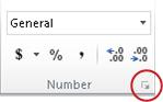
  2. On the Home tab, in the Number group, click the Dialog Box Launcher next to Number.
    Dialog Box Launcher in Number group
  3. In the Category box, click the number format that you want to use.
    For this procedure to complete successfully, make sure that the numbers that are stored as text do not include extra spaces or nonprintable characters in or around the numbers. The extra spaces or characters sometimes occur when you copy or import data from a database or other external source. To remove extra spaces from multiple numbers that are stored as text, you can use the TRIM function or CLEAN function. The TRIM function removes spaces from text except for single spaces between words. The CLEAN function removes all nonprintable characters from text.
Top of Page

Turn off Error Checking

With error checking turned on in Excel, you see a small green triangle if you enter a number into a cell that has text formatting applied to it. If you don’t want to see these error indicators, you can turn them off.
  1. Click the File tab.
  2. Under Help, click Options.
  3. In the Excel Options dialog box, click the Formulas category.
  4. Under Error checking rules, clear the Numbers formatted as text or preceded by an apostrophe check box.
  5. Click OK.


    www.iptindia.com

Merge cells

Merge cells

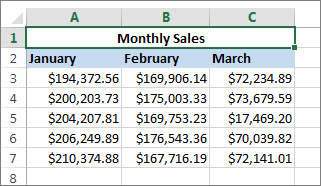
Merging combines two or more cells to create a new, larger cell. This is a great way to create a label that spans several columns. For example, here cells A1, B1, and C1 were merged to create the label “Monthly Sales” to describe the information in rows 2 through 7.
Merge cells above other cells
  1. Important: Make sure the data you want to end up in the merged cell is in the upper-left cell. All data in the other merged cells will be deleted. To keep any data from the other cells, copy it to another spot in the worksheet before you merge.
  1. Click Home > Merge & Center.
Merge and Center button
If Merge and Center is dimmed, make sure you’re not editing a cell and the cells you want to merge aren’t inside a table.
Tip:  To merge cells without centering, click the arrow next to Merge & Center, and then click Merge Across or Merge Cells.
If you change your mind, you can always split the cells you merged.

Advanced Excel Training

Quick start: Sort data in an Excel worksheet

Quick start: Sort data in an Excel worksheet

Quick start: Sort data in an Excel worksheet

When you sort information in a worksheet, you can see data the way you want and find values quickly. You can sort a range or table of data on one or more columns of data; for example, you can sort employees first by department and then by last name.

How to sort in Excel?

Icon image Select the data that you want to sort   
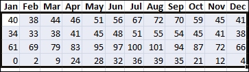
  • Select a range of data, such as A1:L5 (multiple rows and columns) or C1:C80 (a single column). The range can include titles (headers) that you create to identify columns or rows.
Example of selected data to sort in Excel
Icon image Sort quickly   
  1. Select a single cell in the column you want to sort.
  2. On the Data tab, in the Sort & Filter group, click A to Z command in Excel that sorts A to Z or smallest number to largest to perform an ascending sort (A to Z or smallest number to largest).
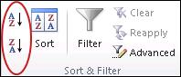
    Sort buttons in the Sort & Filter group on the Data tab in Excel
  3. Click Z to A command in Excel that sorts Z to A or largest number to smallest to perform a descending sort (Z to A or largest number to smallest).
Icon image Sort by specifying criteria   
Use this technique to choose the column you want to sort, plus other criteria such as font or cell colors.
  1. Select a single cell anywhere in the range that you want to sort.
  2. On the Data tab, in the Sort & Filter group, click Sort.
    Sort command in the Sort & Filter group on the Data tab in Excel
    The Sort dialog box appears.
  3. In the Sort by list, select the first column on which you want to sort.
  4. In the Sort On list, select either Values, Cell Color, Font Color, or Cell Icon.
  5. In the Order list, select the order that you want to apply to the sort operation — alphabetically or numerically ascending or descending (that is, A to Z or Z to A for text or lower to higher or higher to lower for numbers

Split text into different columns with the Convert Text to Columns Wizard

Split text into different columns with the Convert Text to Columns Wizard

Split text into different columns with the Convert Text to Columns Wizard

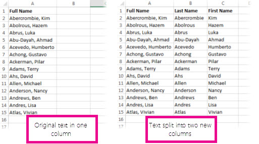
You can take the text in one or more cells, and spread it out across multiple cells. This is called parsing, and is the opposite of concatenating, where you can combine text from two or more cells into one cell. For example, if you have a column of full names, you can split that column into separate first name and last name columns, like this:
Before and after of text split into different columns
Go to Data > Text to Columns, and the wizard will walk you through the process. Here’s a full breakdown of how it works:
  1. Select the cell or column that contains the text you want to split.
    Note:  Select as many rows as you want, but no more than one column. Make sure there’s enough empty columns to the right so nothing over there gets overwritten. If you don’t have enough empty columns, add them.
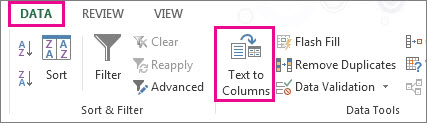
  2. Click Data >Text to Columns.
    Click the Data tab, and then click Text to Columns
  3. This starts the Convert Text to Columns Wizard. Click Delimited > Next.
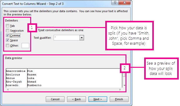
  4. Check Space, and clear the rest of the boxes, or check Comma and Space if that is how your text is split (Smith, John, with a comma and space between the names). You can see a preview of your data in the Data preview window.
    Step 2 in the Convert Text to Columns Wizard
  5. Click Next.
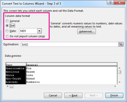
  6. In this step, you pick the format for your new columns, or you can let Excel do it for you. If you want to pick your own format, select the format you want, such as Text, click the second column of data in the Data preview window, and click the same format again. Repeat for all the columns in the preview window.
    Step 3 in the Convert Text to Columns Wizard
  7. Click the Collapse Dialog Box button image button to the right of the Destination box to collapse the dialog box.
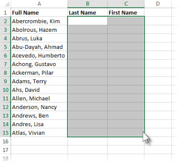
  8. Select the cells in your workbook where you want to paste your split data. For example, if you are dividing a full name into a first name column and a last name column, select the appropriate number of cells in two adjacent columns.
    Select the cells where you wnt to paste your split cells
  9. Click the Expand Dialog Box button image button to expand the dialog box, and then click Finish.

Split text into different columns with the Convert Text to Columns Wizard

Split text into different columns with the Convert Text to Columns Wizard


Split text into different columns with the Convert Text to Columns Wizard

You can take the text in one or more cells, and spread it out across multiple cells. This is called parsing, and is the opposite of concatenating, where you can combine text from two or more cells into one cell. For example, if you have a column of full names, you can split that column into separate first name and last name columns, like this:
Before and after of text split into different columns
Go to Data > Text to Columns, and the wizard will walk you through the process. Here’s a full breakdown of how it works:
  1. Select the cell or column that contains the text you want to split.
    Note:  Select as many rows as you want, but no more than one column. Make sure there’s enough empty columns to the right so nothing over there gets overwritten. If you don’t have enough empty columns, add them.
  2. Click Data >Text to Columns.
    Click the Data tab, and then click Text to Columns
  3. This starts the Convert Text to Columns Wizard. Click Delimited > Next.
  4. Check Space, and clear the rest of the boxes, or check Comma and Space if that is how your text is split (Smith, John, with a comma and space between the names). You can see a preview of your data in the Data preview window.
    Step 2 in the Convert Text to Columns Wizard
  5. Click Next.
  6. In this step, you pick the format for your new columns, or you can let Excel do it for you. If you want to pick your own format, select the format you want, such as Text, click the second column of data in the Data preview window, and click the same format again. Repeat for all the columns in the preview window.
    Step 3 in the Convert Text to Columns Wizard
  7. Click the Collapse Dialog Box button image button to the right of the Destination box to collapse the dialog box.
  8. Select the cells in your workbook where you want to paste your split data. For example, if you are dividing a full name into a first name column and a last name column, select the appropriate number of cells in two adjacent columns.
    Select the cells where you wnt to paste your split cells
  9. Click the Expand Dialog Box button image button to expand the dialog box, and then click Finish.